
How many times have you downloaded some account data from a bank, credit card company, or some other source, hoping to work with it as a spreadsheet, only to find that the information is arranged in such a way as to render it nearly useless without a lot of manual effort?
In this post, the first in a series to cover this topic, we will explore one approach using Power Query to transform a typical download into a proper table suitable for analysis in Excel. We will focus on a small portion of the larger Invoice data set to describe this approach. Subsequent posts will demonstrate techniques that could make the query’s M code more readable, including how commenting the query can serve to document the query steps for future reference, building and applying custom functions, and dealing with repeating groups of data in a download. Some of the steps we will build can be done from the U.I. while others will require manually editing in the Advanced editor.
Download the starting file here to follow along.
Let’s dive in…
Getting Started – Our Goal & Approach
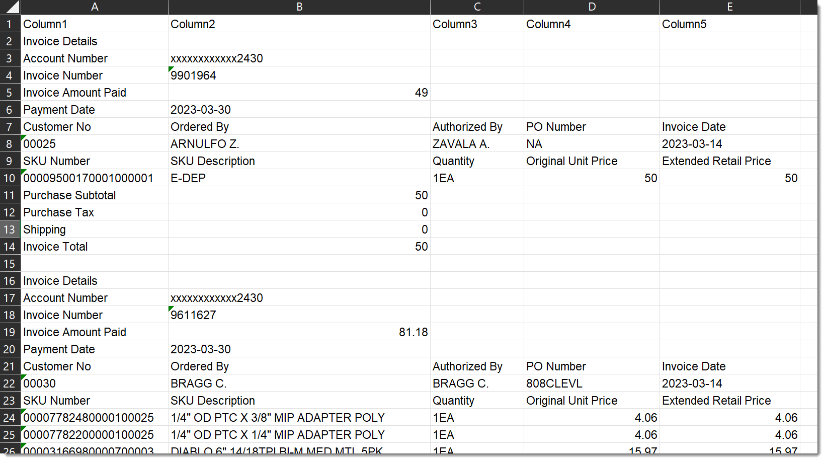
The image below is an excerpt from a larger data set containing over 4,000 rows representing many Invoices. It is clearly NOT a table that we can use as-is for analysis. But within this data, notice there are 4 inner tables. Two of them have a horizontal orientation and two have a vertical orientation. The last inner table has 4 rows, but two of those data points represent values that can be calculated from the raw data, so we won’t include them in our final table.
Our overall approach will be to:
- load the sample data into Power Query
- define each inner table
- transform vertically-oriented tables to be horizontally-oriented
- clean up names in the APPLIED STEPS well
- assemble all 4 of these inner tables into one contiguous table with no blank rows, as shown below
- load the completed table to a worksheet

Step 1: Loading the data into Power Query
Our raw data has already been converted to an Excel table (Ctl + t) and is ready to be loaded into Power Query. Select a cell within the data table and choose the Data>From Table/Range option in Excel’s
Get & Transform Data section on the Data tab.
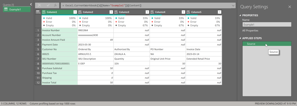
**If you end up with an extra step called ‘Changed Type’, simply click the ‘x’ next to it to delete that step. My default setting for ‘Type Detection’ may be different than yours.
Step 2: Defining the first inner table
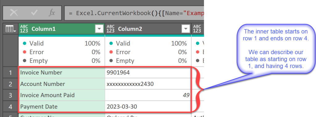
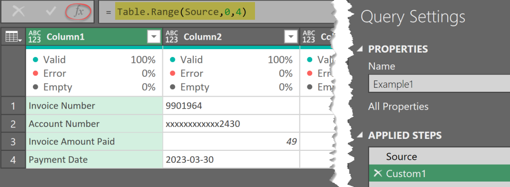
The first inner table begins on the row where Column1 = “Invoice Number” and it ends on the row where Column1 = “Payment Date”. In this example, that equates to rows 1 – 4.
Power Query has a function named Table.Range() to select a subset of rows from a larger table. This function takes 3 arguments:
- table: the query step name representing the whole table containing the inner table
- offset: the number of rows from the first row of the table to the first row of the inner table
- count: the number of rows of the inner table
- Click on the fx button and type the following into the formula bar =Table.Range(Source,0,4)
This tells Power Query we want identify a range of rows within the ‘Source‘ table beginning 0 rows from the top and including 4 rows. - hit Enter or click the checkmark to save the change.
Power Query assigns the step name ‘Custom1’ to our first inner table. We’ll go back and change the name to something more meaningful later on.
Step 3: Transform the first Inner table
Our first inner table is organized vertically, meaning the values sit alongside the labels rather than beneath them. To address this, we’ll need to rotate it 90 degrees, shifting the row headings to the top row of the table, which we can then promote to become the actual column headings. Additionally, it’s important to trim any unnecessary rows that don’t provide valuable information to the table.
- On the Transform tab, click the ‘Transpose’ function.
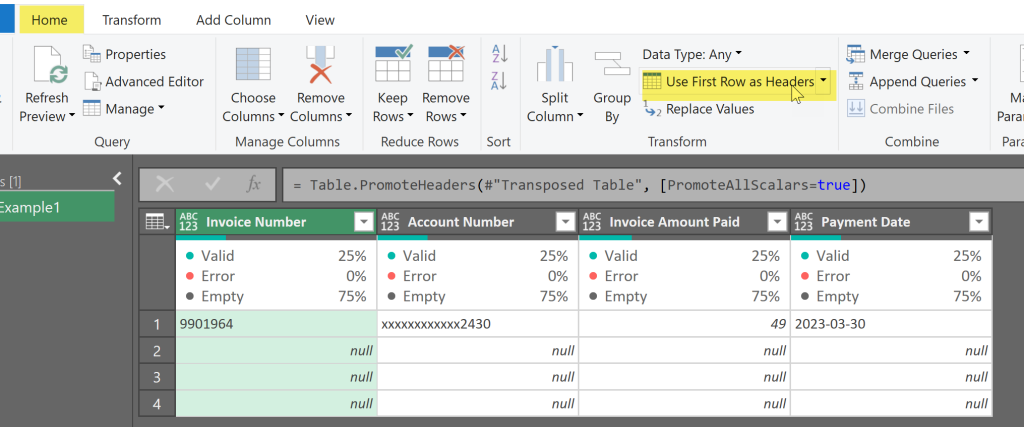
The table’s row headings are now the first row of the table. - Go to the Home tab,
- Click on ‘Use First Row as Headers’.
After promoting the headers, we can see that there is only a single row containing data at this point.
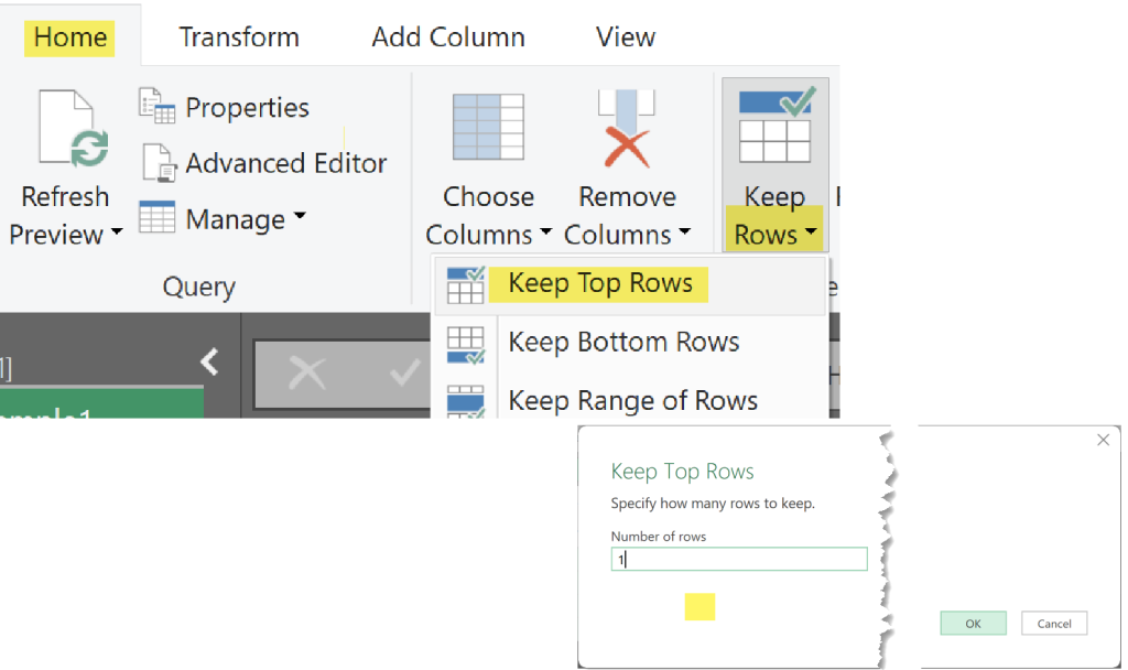
So let’s remove the empty rows. - Click the arrow on ‘Keep Rows’ option
- Click on ‘Keep Top Rows’
- Enter a 1 in the dialog box then click OK
Defining the remaining inner tables
I’ve gone ahead and added the steps to define and transpose the remaining tables. The M code generated is shown below. You could try to follow the code and do these steps on your own. Or you could copy the code and paste it over the existing code in the Advanced Editor and click the Done button.
let
Source = Excel.CurrentWorkbook(){[Name="Example1"]}[Content],
Custom1 = Table.Range(Source,0,4),
#"Transposed Table" = Table.Transpose(Custom1),
#"Promoted Headers" = Table.PromoteHeaders(#"Transposed Table", [PromoteAllScalars=true]),
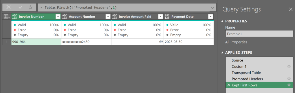
#"Kept First Rows" = Table.FirstN(#"Promoted Headers",1),
Custom2 = Table.Range(Source,4,2),
#"Promoted Headers1" = Table.PromoteHeaders(Custom2, [PromoteAllScalars=true]),
Custom3 = Table.Range(Source,6,2),
#"Promoted Headers2" = Table.PromoteHeaders(Custom3, [PromoteAllScalars=true]),
Custom4 = Table.Range(Source,9,2),
#"Transposed Table1" = Table.Transpose(Custom4),
#"Promoted Headers3" = Table.PromoteHeaders(#"Transposed Table1", [PromoteAllScalars=true]),
#"Kept First Rows1" = Table.FirstN(#"Promoted Headers3",1)
in
#"Kept First Rows1"To catch up using the code provided –
- Copy the code from the block, above.
- Go to the Home tab
- Click on ‘Advanced Editor’.
- Select all the code
- Paste the new code over the selection
- Click Done
Step 4: Renaming Applied Steps
In the code block, above, the highlighted lines of code show the steps where each of our 4 inner tables are materialized. You can also see the names and each table in the images, below. The auto-assigned step names merely mimic the function called at these steps but don’t have any semantic meaning. Let’s change these names to better reflect what’s being returned in each of these steps.
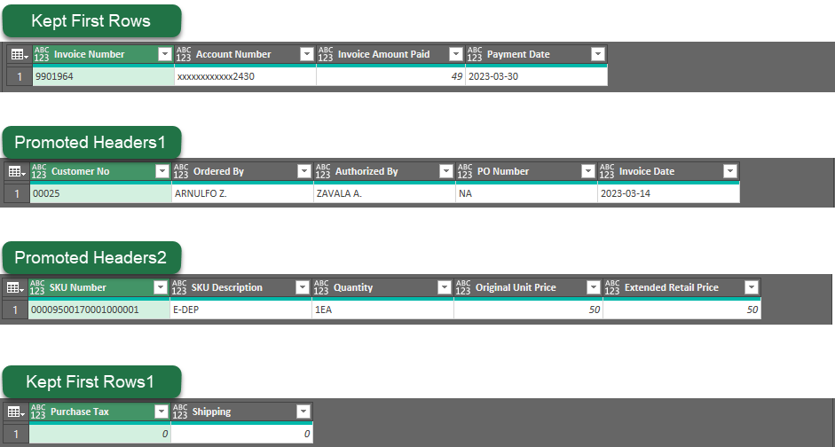
Renaming the steps is very easy. And doing so in the APPLIED STEPS area lets Power Query update any subsequent steps automatically. We will revisit the benefits of a good naming convention in a future post. I tend to use camel-case names with no spaces or underscore characters, that reflect what is happening at or being returned at each step. Let’s change the names for the steps that materialize our inner tables:
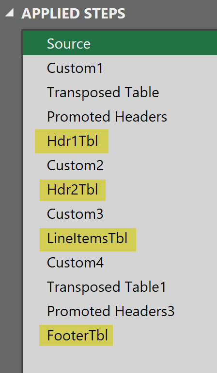
- Right-click on each step and choose the Rename option from the context menu
- type over the existing name with the corresponding names found in the below list:
- Kept First Rows → Hdr1Tbl
- Promoted Headers1 → Hdr2Tbl
- Promoted Headers2 → LineItemsTbl
- Kept First Rows1 → FooterTbl
Sensible names makes it easier to refer to each table for the next step. Looking back at the APPLIED STEPS, it’s now much easier to identify the steps which return our inner tables.
Step 5: Combining the inner tables
Our next goal is to assemble all of the inner tables, side-by-side, to form a single contiguous table containing only rows with relevant content. Power Query’s Table.Combine() function will do just that.
Table.Combine() takes a list of tables to combine as a single argument. The proper syntax for that is:
Table.Combine( {table1, table2, table3, table4} )
Notice how the names of the 4 tables are enclosed inside curly braces({}) to denote a list.
- Click on the fx button and double-click the FooterTbl value in the address bar to replace it
- Type the following Table.Combine( {Hdr1Tbl, Hdr2Tbl, FooterTbl, LineItemsTbl} ) after the ‘=’ sign
- Hit Enter or click the checkmark to save the change
After you enter this function, you should see the following:

This function stacked each of the tables on top of each other aligning columns where the names have an exact match. Columns that have no match in any other table are added off the right. Each of our 4 tables have unique column names, so they will be stacked as separate columns to the right. It also means that there will be rows in the resulting table to eliminate because they don’t contain useful data.
Step 6: Cleaning up the final table
Referring to the above image, we can see that there is really just a single row of data for this invoice. If we could get the values from each of the 1st three inner tables to drop down to the last row, we would be able to eliminate the top 3 rows to clean up the whole table.
Power Query offers a transform called Table.FillDown() which does just that; it copies a non-null value in one cell into all of the cells beneath (or above) it until it hits another non-null cell.
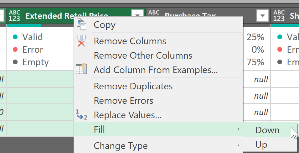
To apply the ‘Fill Down’ function:
- select all of the columns that have any blanks beneath them
- All columns except the last 4 columns
- right-click in one of the selected column headings
- choose Fill, then choose Down
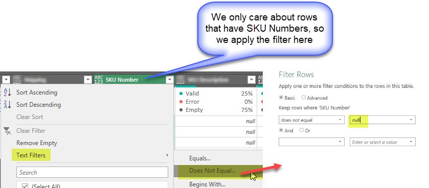
Now we can remove all the rows that have no data by applying a filter to the ‘SKU Number’ column:
- Click the filter button on the SKU Number column
- Choose Text Filters
- Then choose Does Not Equal..
- Enter ‘null‘ as shown
- Then click OK
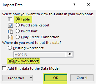
And to complete our exercise:
- Select the Home tab
- click on the ‘Close & Load To…
- select options as shown at left
- click OK to load our newly completed table to a new worksheet

Conclusion
In this exercise, we have taken a small data sample, identified 4 inner tables hiding within that data, broke them out and re-assembled them into a viable data table projected on a worksheet. We used a mix of build-in ribbon commands and manually entering functions in the formula bar. And we renamed some steps to make it easier to refer to each of our inner tables.
The result isn’t a very useful data set, but in the next post in this series, we will work with more invoices and learn to replace hard-coded values in our functions with dynamic references that will allow us to build a custom function to handle any number of invoices.
You can download the completed file here.
Check back for the next post…