
This is the 2nd post in a series featuring examples of how to use Power Query to transform the data in a typical downloaded account statement file into something that can easily be analyzed in an Excel workbook.
In Part 1, we looked at one approach to transforming the data for one representative invoice record. In this article, we will build on those ideas and cover the following:
- working with the Power Query Advanced Editor
- replacing hard-coded arguments with dynamic references
- nesting functions
- the benefits of naming conventions
Download the starting file here to follow along.
Let’s dive in…
Background
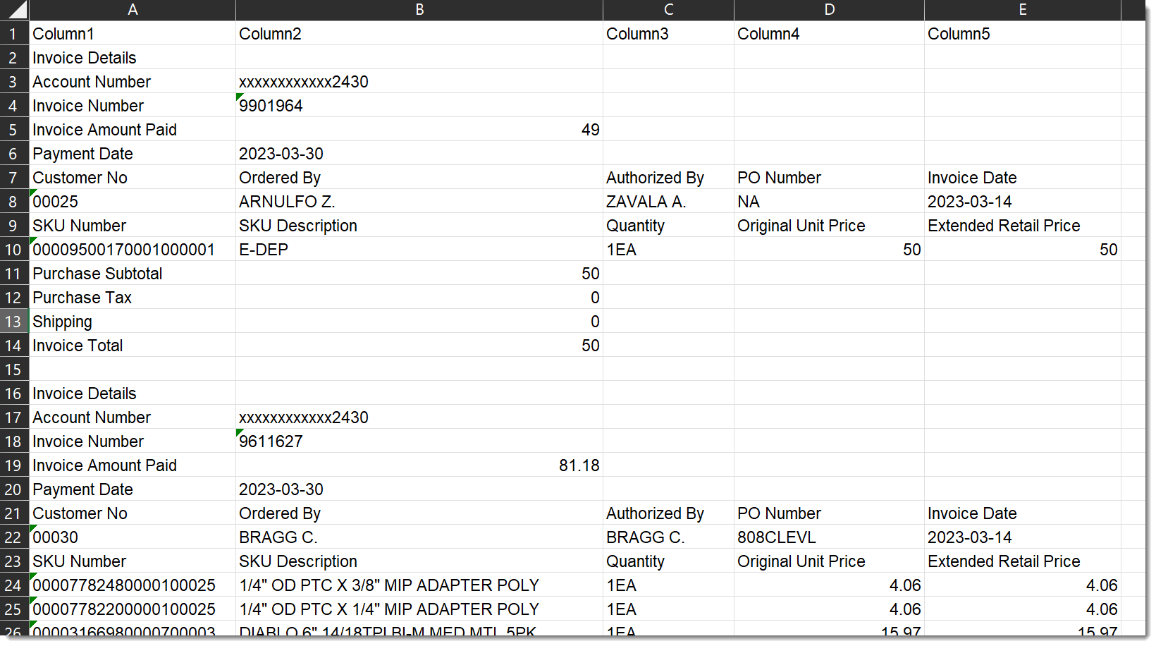
The data we worked with last time was related to a single invoice. The steps used to transform that data will only work on that one specific invoice because we hard-coded some values in the query steps. In this article, we will work with 2 invoices to learn how to improve the query code to handle an unknown number of invoices in the future.
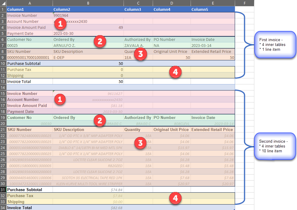
The image above shows the information for 2 separate invoices. The structure for each invoice is consistent aside from the fact that the 2nd invoice has multiple line items where the first invoice had only one. The approach used for the first example relied on defining the extents of the inner tables using hard-coded numbers we could see from the static example. This won’t work for data sets that can vary in size.
Introducing List.PositionOf()
We used Table.Range(Source, 0, 4) to return a range from the Source table (whole data set) which starts on the first row and extends 4 rows. But consider the 3rd inner table between these two invoices. The first invoice has only 1 SKU number while the second invoice has 10 SKUs. Using hard-coded arguments doesn’t allow for flexible ranges. We need a way to dynamically determine the start/end rows for each table.
Power Query has a function called List.PositionOf() which returns the offset at which some value is found within some list. Let’s leverage this function by writing some M code in the Advanced Editor.
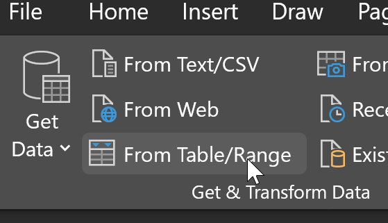
- Create a new query by clicking anywhere within the data table
- On the Data tab, choose ‘From Table/Range’
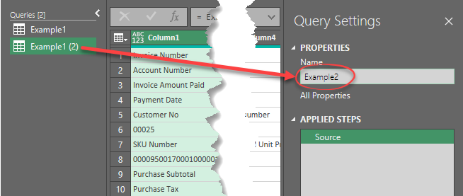
**If you end up with an extra step called ‘Changed Type’, simply click the ‘x’ next to it to delete that step. My default setting for ‘Type Detection’ may be different than yours. - Edit the name of the new query in the Query Settings pane to be Example2
Using the Advanced Editor
Click the ‘Advanced Editor’ button on the Home tab. The editor window opens with some M code in it already. The first step in this query is named ‘Source’. This represents the whole data set from our worksheet; in our case, just 2 invoices. Let’s add some code to see what the List.PositionOf() functions return for position.
When editing in the Advanced Editor, we have to assign names to each step and remember to terminate each line with a comma (,) for all but the last line before the ‘in’ step. Assigning meaningful names to each step can help anyone who works with this code in the future, and avoiding spaces and underscores in those names will make it easier to work with them down the road.
**Remember: Power Query is case-sensitive
Step 1: Adding Code to find Positions
- On the Home tab, click on ‘Advanced Editor’ so we can begin our manual modifications
- Enter a comma at the end of the Source line, and hit enter to start a new line.
- Copy and paste, or type these lines into the editor beneath the Source step, but before the ‘in’ line
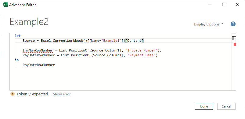
- InvNumRowNumber = List.PositionOf(Source[Column1], “Invoice Number”),
- PayDateRowNumber = List.PositionOf(Source[Column1], “Payment Date”)
**NOTE: if you copy/paste the code and get an error, it could be that the double quotes (“)were replaced with some strange characters from the web browser. Delete each instance and type them in manually.
- Replace ‘Source’ on the last line with ‘
PayDateRowNumber‘ then click the Done button.
The query now returns the result found from step PayDateRowNumber: 3. If you modify the query and replace PayDateRowNumber with InvNumRowNumber you would see it returns the number 0.
The query returns the number 3 as the result of this query because the PayDateRowNumber step calculates the position using a zero-based index.
The Advanced Editor will warn you if there is some problem in your code. The red underlines give you a clue as to where problems are. And the message below the code window can help you figure out what’s wrong.
Forgetting the comma at the end of the first line results in red line indicating that something is wrong.
Skipping a line after the ‘Source’ step to add white space can help readability of the code.
Step 2: Defining the range Dynamically
Now that we know the positions of these important rows, we can use the Table.Range() function again to select a range, but rather than hard-coding the row number arguments, we’ll use our new calculated values as arguments making the function dynamic.
InvNumRowNumber returns 0, so we can use that as the first argument. However, PayDateRowNumber returns a 3 where we need a 4 as our argument. No problem. We’ll just add 1 to it to account for the Zero-based row numbering. Re-open the Advanced Editor to make the following changes:
- Type a comma (,) at the end of the ‘
PayDateRowNumber‘ line and hit Enter to start a new line - Type Hdr1Range = Table.Range(Source, InvNumRowNumber, PayDateRowNumber + 1)
- ‘Hdr1Range‘ is a suitable name for this transform, but it could be anything you want.
- After the ‘in’ expression, replace ‘PayDateRowNumber‘ with ‘Hdr1Range‘
- Click the Done button
We’ve now defined a table range and assigned it to the variable ‘Hdr1Range‘. But it has a vertical orientation and we need it to be horizontal. The Table.Transpose() function introduced in the last post accomplishes this.
We could add it as a new step, but let’s wrap it around the Table.Range function to do it all in one step as shown below.
- modify the Hdr1Range step as follows –
- change it from: Table.Range(Source, InvNumRowNumber, PayDateRowNumber + 1)
to - this: Table.Transpose( Table.Range(Source, InvNumRowNumber, PayDateRowNumber + 1) )
- change it from: Table.Range(Source, InvNumRowNumber, PayDateRowNumber + 1)
- click the Done button to see the results
let
    Source = Excel.CurrentWorkbook(){[Name="Example1"]}[Content],

    InvNumRowNumber = List.PositionOf(Source[Column1], "Invoice Number"),
    PayDateRowNumber = List.PositionOf(Source[Column1], "Payment Date"),
    Hdr1Range = Table.Transpose(
                            Table.Range(Source, InvNumRowNumber, PayDateRowNumber + 1)
                                )
in
    Hdr1Range
Step 3: Cleaning up the resultant table
The last two steps to materialize this inner table can be done using the U.I. They are –
- promote the headers, and
- remove the rows that don’t contain data
We can add these next steps using the commands on the Home tab:
- click on the ‘Use First Row as Headers‘
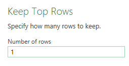
- click the arrow on the ‘Keep Rows‘ option, then click ‘Keep Top Rows‘
- enter a 1 in the dialog box
- click OK
After this last change, we have our first inner table defined, transposed to a vertical orientation with no empty rows.

Using the UI means Power Query assigns step names that usually contain spaces which means they must start with a pound sign (#) and be wrapped in double quotes (“). It makes for messy code, so I often take the time to clean up the names myself. Let’s go back into the editor to see if we can improve on the code written for us after adding the last steps.
Edit the code to consolidate the last two steps into one, and assign a more obvious step name.
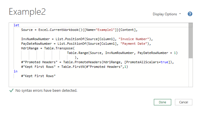
- combine the last 2 steps by nesting the Table.PromoteHeaders() function inside the Table.FirstN() function
- change Table.FirstN(#”Promoted Headers”,1)
to - Table.FirstN( Table.PromoteHeaders(Hdr1Range, [PromoteAllScalars=true]),1)
- change Table.FirstN(#”Promoted Headers”,1)
- Delete the line –
“Promoted Headers” = Table.PromoteHeaders(Hdr1Range, [PromoteAllScalars=true]), - Rename the last step from #”Kept First Rows” to ‘Hdr1Tbl’
- Change the line after the ‘in’ expression from #”Kept First Rows” to ‘Hdr1Tbl’
- Click the Done button to save your changes
let
    Source = Excel.CurrentWorkbook(){[Name="Example1"]}[Content],

    InvNumRowNumber = List.PositionOf(Source[Column1], "Invoice Number"),
    PayDateRowNumber = List.PositionOf(Source[Column1], "Payment Date"),
    Hdr1Range = Table.Transpose(
                            Table.Range(Source, InvNumRowNumber, PayDateRowNumber + 1)
                                ),
    Hdr1Tbl = Table.FirstN(
                            Table.PromoteHeaders(Hdr1Range, [PromoteAllScalars=true]),
                            1)
in
    Hdr1Tbl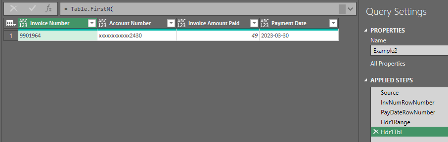
With the last changes, our query screen looks neater, with step names that are meaningful.
Document code with Comments
Another advantage of using the Advanced Editor is that you can easily include comments throughout the code. Comments can be added as –
- Single-Line: are created by starting the line with two forward slashes (
//). Anything following the//on that line is treated as a comment. - Multi-line comments: are enclosed within
/*and*/and can span multiple lines. Anything between/*and*/is treated as a comment. - In-line comments: are created on the same line as your code. Anything following
//on a line of code is treated as a comment.
I’ve added a comment line to document what the block of code is doing. Notice how the comment text is green, indicating that it is not executable code. Consider using comments to enhance the readability and maintainability of your queries.
let
    Source = Excel.CurrentWorkbook(){[Name="Example1"]}[Content],

    //Grab and rotate the first inner table, promote col hdgs and drop null rows
    InvNumRowNumber = List.PositionOf(Source[Column1], "Invoice Number"),
    PayDateRowNumber = List.PositionOf(Source[Column1], "Payment Date"),
    Hdr1Range = Table.Transpose(
                            Table.Range(Source, InvNumRowNumber, PayDateRowNumber + 1)
                                ),
    Hdr1Tbl = Table.FirstN(
                            Table.PromoteHeaders(Hdr1Range, [PromoteAllScalars=true]),
                            1)
in
    Hdr1Tbl
Transform the remaining inner tables
The same techniques can be used to define the remaining three inner tables. I’ve gone ahead and finished adding the code and comments in the Advanced Editor. The Power Query window shows all of the steps with care taken to name each step.
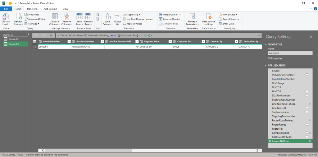
You can download the completed file here.
Conclusion
In this exercise we looked at a data set containing multiple invoice records to illustrate why making functions dynamic is important when building queries that will be used repeatedly. We made extensive use of the Advanced Editor, including nesting functions in a single step, adding spacing between logical groups of steps, documenting the steps with comments, and applying meaningful step names throughout the query.
In the next article, we will take what we’ve worked on here to the next level using nested queries to further consolidate our code on our way to creating a custom function that will finally allow us to handle the larger data set with many invoice records. Check back for Part 3 soon.