
This is the 4th post in a series featuring examples of how to use Power Query to transform the data in a typical downloaded account statement file into something that can easily be analyzed in an Excel workbook. In Part 1, we looked at one approach to transforming the data for one representative invoice record. In Part 2 we improved on the query by replacing the hard-coded arguments with dynamic references to allow the query to adapt to variability in the source data and we made extensive use of the Advanced editor, including adding spacing between logical groups of steps, documenting the steps with comments, and applying sensible step names throughout the query. In Part 3 we further cleaned up the M code by nesting multiple queries inside of the main query to reduce the visible number of Applied Steps, we applied helpful names to our new steps and added more comments to document what we were doing for future reference.
In this last exercise, we will be working against a much larger data set, with over 4,000 rows of data representing more than 220 Invoices. Our goals are as follows:
- update the query we finished with in exercise 3 to account for a different layout of the raw data
- convert our query from the last exercise into a custom function
- learn how to isolate each Invoice record so we can use our custom function to process it
- process the entire data set by invoking our new function
To accomplish all of this, the post will be much longer than most. But if you stick it out, I think it will be worth the effort. We will again be working largely in the Advanced Editor. And we will be applying many of the same ideas we covered in previous exercises to reinforce them.
So let’s get started!
Download the starting file here.
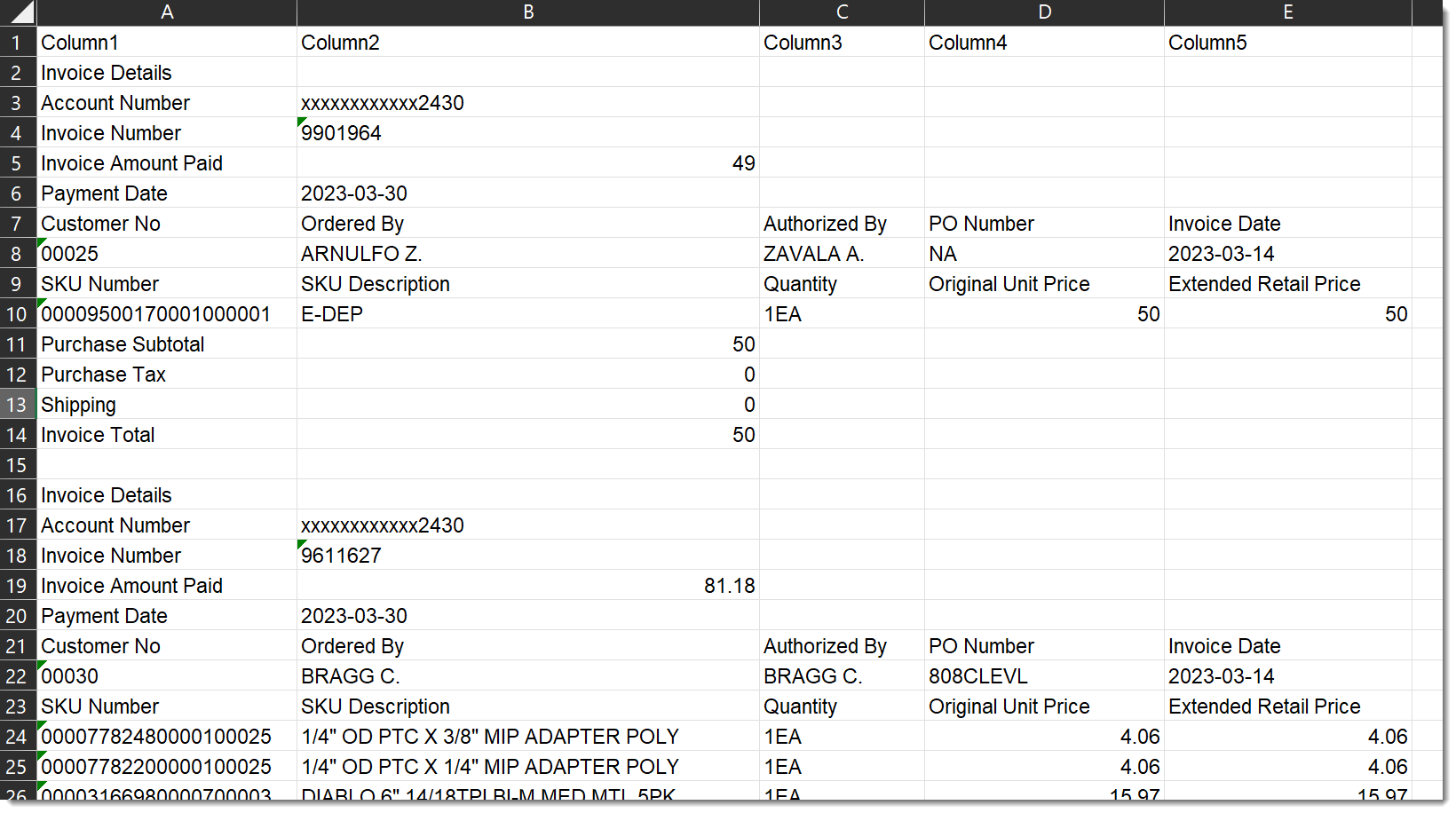
Our New Data Set
Up until now, we have only see 2 Invoice records from the larger data set which I had modified slightly to make it a bit easier to work with as we eased into the examples.
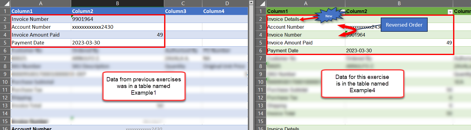
The new data set has one extra row (Invoice Details) for each Invoice record. Also notice that the Account Number and Invoice Number rows have been reversed from our original examples. So we will need to deal with these differences before we move on to the good stuff!
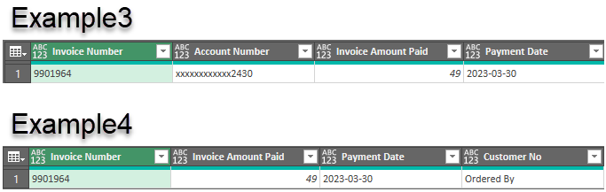
Make note that the small data set is in a table named ‘Example1’, so the Source step in the Example3 query starts with = Excel.CurrentWorkbook(){[Name=”Example1“]}[Content]. When we duplicate it to make Example4, we have to point the Source to the new table containing all the sample data. The new table name is Example4.
The rows that have the label ‘Invoice Details’ don’t have any value in the data so we can filter those rows out and forget about them. But the re-ordered rows will break our existing query because the approach was to define the Hdr1Tbl table as starting on the row where we find ‘Invoice Number’ and ending on the row where we find ‘Payment Date’. Under that definition, the ‘Account Number’ row would be excluded from the table. We need to modify the nested query such that it defines the first inner table as starting on the ‘Account number’ row. This will be good practice…
Step 1: Create the Example4 query
Open the Power Query Editor to make a copy of the Example3 query we used in the last exercise. On the ribbon, click Data, then click Queries & Connections. (hint: if you right-click on the ‘Queries & Connections’ command, you can easily add the command to your Quick Access Toolbar! You DO use that, right?)
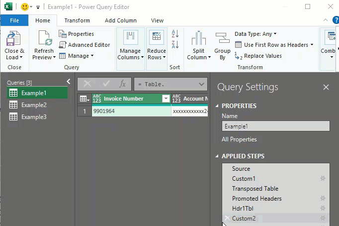
Now we have a new query object to modify without sacrificing our previous work. In the Applied Steps, click on the Source step to edit the table name to connect to.
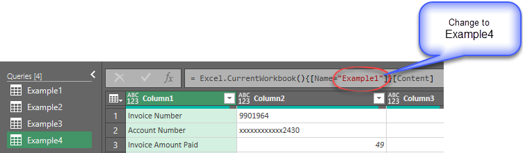
After changing the name and hitting Enter, the ‘Invoice Details’ row appears in the grid confirming that you are connected to the new data set.
Dealing with different data structure
Step 2: Filter out the ‘Invoice Details’ rows
Let’s drop all the rows where Column1 = ‘Invoice Details’ by applying a Text Filter on that column.
- **Click on the Source step under Applied Steps for Example4
- Click on the Column Menu (filter button) on the right edge of Column1
- Click ‘Does Not Equal…’
- Fill out the rest of the options as shown below
** REMEMBER THAT Power Query is case sensitive **
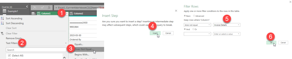
After applying the filter, the Applied Steps shows a new step after the Source step. It’s not a great name for 2 reasons: it has a space in the name, and we don’t know what the filter is doing.
Let’s edit the step name to something better.
- Right-click on the step name in the Applied Steps and choose Rename
- Edit the name to be ‘FilterOutInvDetails’
- Then, hit Enter
Changing the step name here rather than in the Advanced Editor, has the advantage of propagating the name change throughout the rest of the query code. Very slick!
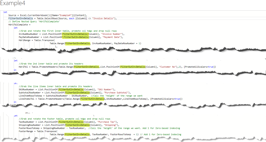
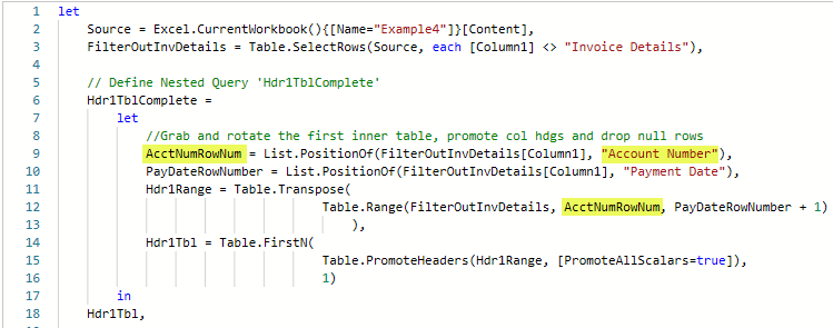
Step 3: Redefine Hdr1Tbl
The current definition of the Hdr1Tbl is explained in the image below. Rearranging the ‘Invoice Number’ and ‘Account Number’ rows in the data set skews the starting row table down by one row which means we not only miss the ‘Account Number’ data, but we pick up the first row from the next table, Hdr2Tbl.
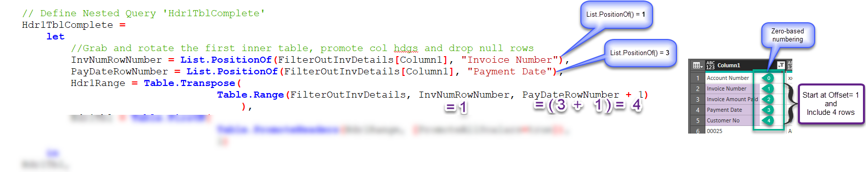
The solution isn’t very hard, and it gives us practice assigning sensible names to our steps. Basically, we don’t care about the position of ‘Invoice number‘ anymore. Instead, we want to get the position of ‘Account Number‘.
Here are the steps to deal with the new arrangement of the data:
- On the Home tab, click on ‘Advanced Editor’
- Click on the ‘Display Options’ dropdown list in the upper right corner of the editor
- Turn on the ‘Display line number’ option
- Edit the code on line # 9 as follows –
change: InvNumRowNumber = List.PositionOf(FilterOutInvDetails[Column1], “Invoice Number“),
to: AcctNumRowNum = List.PositionOf(FilterOutInvDetails[Column1], “Account Number“), - Edit the code on line # 12 as follows –
change: Table.Range(FilterOutInvDetails, InvNumRowNumber, PayDateRowNumber + 1)
to: Table.Range(FilterOutInvDetails, AcctNumRowNum, PayDateRowNumber + 1) - Click the Done button to save your changes
- Under Applied Steps, click on the last step, ‘InvoiceTblDone’ and there should be no errors
Creating Groups of Invoice rows
Our Example4 query extracts and transforms 4 inner tables within the first Invoice record of our data into a single, contiguous table with only column headings. Even though Example4 data has many Invoice records, our query is still only seeing the first Invoice record. Stated differently –
Query Example4 will perform these steps on the first Invoice record in the data set.
Our next challenge will be to find a way to present only 1 Invoice ‘record’ at a time so we point the query at it.
The ‘Group By’ transform
Power query has a transform called Table.Group() which is familiar to many for its ability to combine data by some common key and present various aggregations such as SUM, MIN, MAX, etc. But there is another use for this transform which will let us ‘combine’ rows by a common key (think ‘Invoice Number’) but instead of using a calculation, we will instruct it to return all the rows from each group. When it does this, it will be returning a table on each row. And that table holds all the rows related to one Invoice. (Many thanks to my colleague Tom Allan for this simple solution!)
For us to be able to group the variable number of rows per Invoice record together, they must have something in common; and they do; the ‘Invoice Number’. But for this to work, the Invoice Number must be on every row related to to the invoice. So we need to add a new custom column to hold the ‘Invoice Number’ value and then perform the grouping.
The image below hints at our approach. We’ll add a new column and if the row label in Column1 = ‘Invoice Number’ then we will fill in the new column’s cell with the value found in Column2.
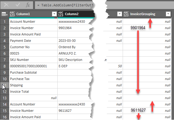
After getting the Invoice number in one cell, we can use Fill Up and Fill Down to spread the Invoice number across all the remaining rows of the Invoice record.
The Table.FillDown() function will copy a non-null value in a cell down a column until it reaches another non-null cell. Consider what will happen if we were to use FillDown in the image above. The 9901964 value will be copied into all the non-null cells beneath it – including row 14 which is a different Invoice record. To prevent that, we can’t have the ‘Account Number’ row’s InvoiceGrouping cell null; it must have a non-null value. Any value will do.
Step 4: Add a custom column to group by
- Under Applied steps, click on the FilterOutInvDetails step
- On the ribbon, select the Add Column tab
- Then, click the Conditional Column
- Click Insert to confirm you wish to insert a new step
- Fill out the dialog box as shown below
- click the ‘Add Clause’ button to add a 2nd condition
- don’t forget to add ‘null’ in the Else branch
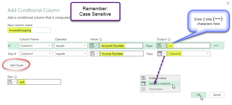
Notice that we are making sure that the ‘Account number‘ row has a non-null value. We’ll go back and replace those values eventually and use the Table.FillUp function to finish populating the column.
- Click OK to close the dialog and create the new column
- Right-click on the InvoiceGrouping column heading and choose Fill>Down
- Click Insert when prompted to add a new step
All the Invoice numbers have propagated down but stop at each ‘Account number‘ row because of the ‘~~’ characters. Now we can replace all the ‘~~’ characters with ‘null’ and then use the Fill>Up function.
- Click the Transform tab on the ribbon and choose Replace Values…
- Click Insert when prompted to add a new step
- In the dialog box, enter ‘~~‘ as the Value To Find, and ‘null‘ as the Replace With value
- Then click OK
- Right-click on the InvoiceGrouping column heading and choose Fill>Up
- Click Insert when prompted to add a new step
We now have the Invoice number written on every row of each respective Invoice record.
Let’s get grouping!
- Click the Group By button on the Transform tab
- Click Insert when prompted to add a new step
- Fill out the dialog box as shown below
- Click OK to finish
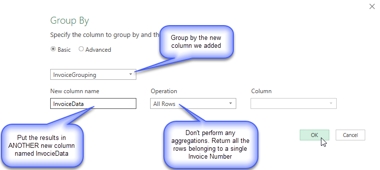
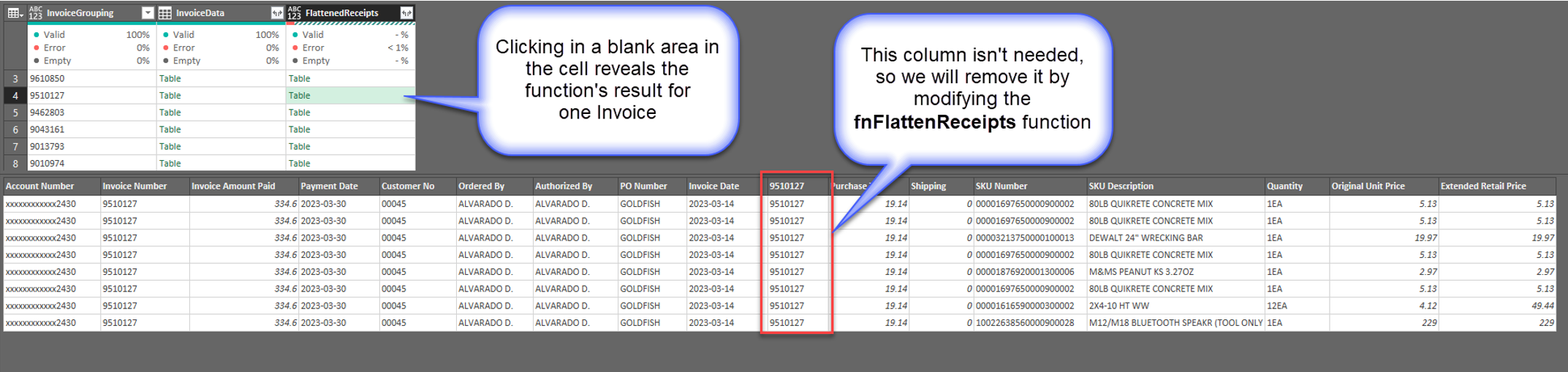
Now, the data have been collapsed so each row in our table holds an Invoice number plus a separate table which includes all the original rows associated with that Invoice number. You can see the contents of the InvoiceData table by clicking on the cell containing the table. (Don’t click on the word ‘Table’, click in a blank area within the cell)
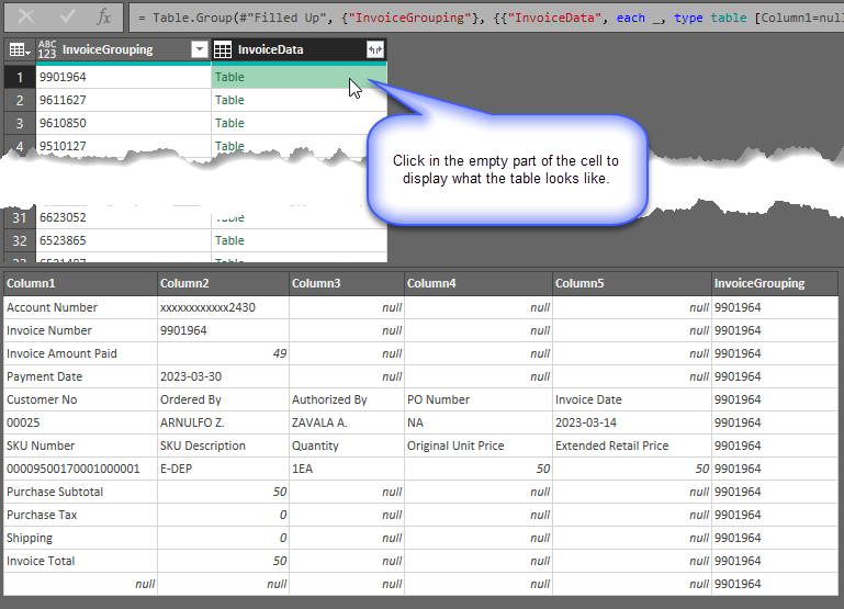
At this point, each row now has in this new column, a single invoice record. The custom function we’ll build will be able to act on each of these tables.
Power Query Custom Functions
In Power Query, a custom function refers to one or more user-defined operations or transformations to be applied to data within a query. You have probably used the SUM() function in Excel, right? We don’t know exactly how it works, but we know what it does; it adds up all the values that are referenced between the parenthesis or its arguments.
In power Query, we can create our own function that performs one or more transforms on some data by passing that data to the function as an argument; in our case, we want to pass all the rows for one Invoice record to our function.
Custom Function Syntax
Below is a simplified example of a custom function named ‘Combine2Words’ which takes 2 arguments and combines them with a hyphen between them.
(argument1, argument2) =>
let
    // Define local variables or intermediate steps here (optional)
    somestepname= argument1 & " - " & argument2
in
    // Return the final result of the function
    somestepname
We can use that function by making a new blank query and calling the function like this:
(argument1 as text, argument2 as text) =>
let
    Source = Combine2Words("Hello", "World")
in
    Source
The result is this:

Knowing that we want to combine two text values, it would be a good idea to let Power Query know that the arguments should be text so it can provide better error handling, IntelliSense recommendations as well as making it easier for anyone looking at the function to understand what is required. We could change the example to look like this: (argument1 as text, argument2 as text) =>.
In the context of what we are working on, our custom function will only have a single argument of the type table which should only contain the rows for a single Invoice record. Our declaration could look like this: (InvTable as table)=>. And the tables that we will use as the argument will be the tables we created when we applied the ‘Group By’ transform, above.
Step 5: Create Our Custom Function Query
Our Example4 query is working up to the ‘Grouped Rows’ step. But if we select any of the remaining steps, we get errors. But that’s ok. The remaining steps will be used to build our function.
Let’s start by duplicating the Example4 query and assigning it the new name.
- Right-click on the Example4 query in the left-hand pane
- Click Duplicate
- Rename the new query to ‘fnFlattenReceipts’ in the right-hand pane
- Click back on the Example4 query
- Right-click on the step named ‘Hdr1TblComplete’ and choose ‘Delete Until End‘
- this removes all the remaining steps from this query
- all of these steps had errors after we preformed the Group By step
- Choose Delete when prompted
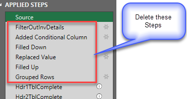
Let’s remove some of the steps from the new fnFlattenReceipts query that are now being handled
in the Example4 query.
- Select the fnFlattenReceipts query
- Delete the following steps from Applied Steps:
- when you hover over a step name, a small ‘x’ icon appears on the left. Click it and confirm the deletion when prompted to delete these steps –
- FilterOutInvDetails
- Added Conditional Column
- Filled Down
- Replaced Value
- Filled Up
- Grouped Rows
- when you hover over a step name, a small ‘x’ icon appears on the left. Click it and confirm the deletion when prompted to delete these steps –
At this point, the fnFlattenReceipts query is reduced to a Source step (which is really just a table!) and all the remaining steps that operate on the rows in that table to convert it to a contiguous table of data. But the Source step is pointing to the WHOLE data set in the Excel worksheet; all 4,000+ rows. We just need to point it to a table which represents a single Invoice record. That’s where the function argument comes into play.
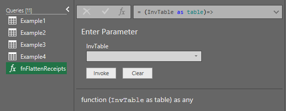
- With the fnFlattenReceipts query still selected, open the Advanced Editor
- Click anywhere inside the code and press Ctl + Home to move the insertion point to the beginning of line #1
- Type the following BEFORE the ‘let’ keyword:
- (InvTable as table)=>
- InvTable is going to be the new ‘Source’ for this query
- Hit Enter to move ‘let’ to the next line
- Delete the whole line #3:
- Source = Excel.CurrentWorkbook(){[Name=”Example4″]}[Content],
- Replace the name ‘Source’ with ‘InvTable’ throughout the rest of the code
- HINT: if you click on the word ‘Source’ on line #10, you should see 11 instances of the word that need to be replaced in the code
- Click ‘Done’ after making the edits
The query has now been converted into a function. Notice that the query window looks totally different than a regular query. And the icon next to the function name indicates that it is a function, not a regular query.
Now let’s apply the function to the grouped tables in the Example4 query.
Step 6: Invoking the function
We will use the new function by adding a new column in which we invoke the custom function. There’s even a special Add Column option just for doing this.
- Select the Example4 query
- From the ‘Add Column’ tab, choose ‘Invoke Custom Function’
- Name the new column ‘FlattenedReceipts’
- Choose ‘fnFlattenReceipts’ as the
Function query - Select the column ‘InvoiceData’ as the InvTable argument
- Click OK to create the new column
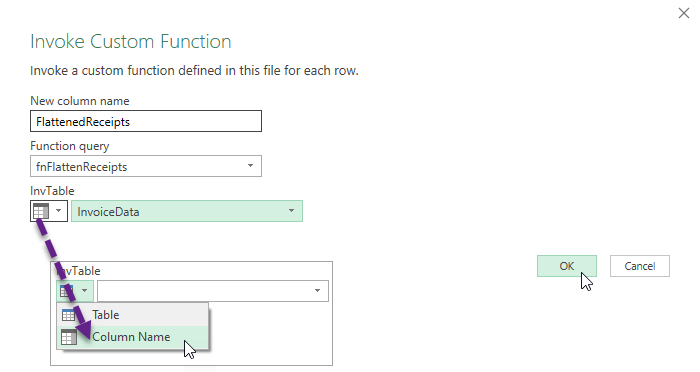
The new column holds tables also. But these tables are the flattened versions of each of the raw data tables in the ‘InvoiceData’ column. The function processed each table individually and stored the results in a new table in each cell of the new column.
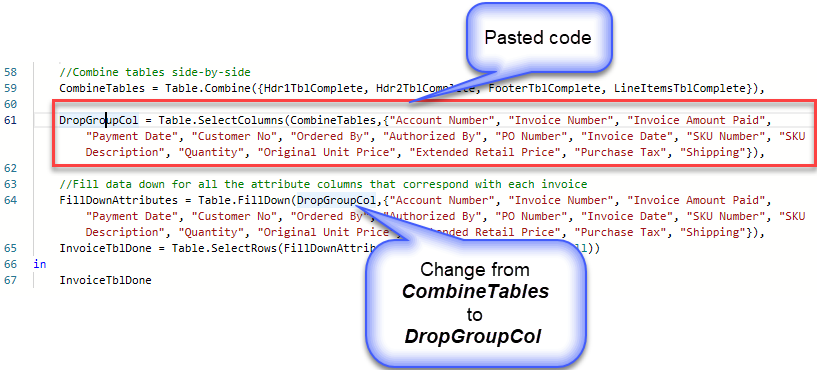
We can see that there is an extra column that we need to remove from the tables. But the name of the column in each individual table will be unique because it’s based on the Invoice number. We can modify the fnFlattenReceipts function to get rid of the unwanted column by telling the query the columns we want to keep by using the Table.SelectColumns() function.
- Right-click on the fnFlattenReceipts function and choose Advanced Editor
- Scroll to the bottom of the code looking for the step name ‘CombineTables’
- this is where the inner table get joined together to form a single flattened table
- Copy the line of code, below, and paste it on the line beneather the ‘CombineTables’ step
- **when copying the code, be sure to include the trailing comma
DropGroupCol = Table.SelectColumns(CombineTables,{"Invoice Number", "Account Number", "Invoice Amount Paid", "Payment Date", "Customer No", "Ordered By", "Authorized By", "PO Number", "Invoice Date", "Purchase Tax", "Shipping", "SKU Number", "SKU Description", "Quantity", "Original Unit Price", "Extended Retail Price"}),- Modify the next step (‘FillDownAttributes’) by changing
‘CombineTables’ to ‘DropGroupCol’ in the Table.FillDown() function- After pasting the code, the ‘FillDownAttributes’ steps is referring to the wrong previous step
- without this change, the ‘DropGroupCol’ step would be ignored
- Click Done to save the changes
‘After changing the code in our custom function, we can go back and ‘peek’ at the tables in the ‘After changing the code in our custom function, we can go back and ‘peek’ at the tables in the ‘FlattenedReceipts’ column to see that the extra column with a column heading of the Invoice number is no longer part of the table.
We can now expand the the column to display all the columns from each row as one contiguous table.
- click on the Table Expansion button to the right of the column heading ‘FlattenedReceipts’

- In the dialog that opens, leave all (Select All Columns) checked
- Make sure the option ‘Use original column names as prefix’ is UNCHECKED
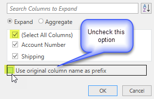
- Click OK to open all the columns
Step 7: Finishing Touches
With all the data transformed from the original data set, we should get rid of any helper columns and then make sure that the data types for the remaining columns are appropriate.
- Select the two columns named ‘InvoiceGrouping’ and ‘InvoiceData’
- click in the column heading of one, hold down the Control key and click in the heading f the other column
- Right-click on one of the headings and choose ‘Remove Columns’, or press your Delete key
- the remaining columns are all we are interested in from the original data set
- Press Ctl + A to select all columns
- Click on the Transform tab and choose the ‘Detect Data Type’ command
- Review the data types assigned to each column by inspecting the icon to the left of the Column name and the display format of the data
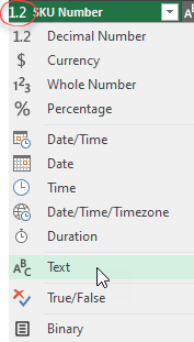
The SKU Number column looks odd because it was assigned the wrong data type; Decimal number. ![]() We can easily change the data type to text to fix how the values are displayed.
We can easily change the data type to text to fix how the values are displayed.
- Click on the icon to the left of the SKU Number column header
- a list of choices appears
- Select the Text option
- When prompted, choose ‘Replace Current’
- This changes the assigned type without adding a new step.
Congratulations! Our function worked!
The output of this query is a well-formed table that we could use as the basis for analysis in Excel. It has no row headings, only column headings. We could still improve upon this, but this post has gone long enough.
Conclusion
We covered a lot in this exercise. In order to use the Group By transform, we had to add a column to group by and get clever to populate it in a way that would allow us to FillDown AND FillUp. We saw how easy it is to duplicate a query to repurpose it. We saw how easy it can be to create a custom function based on all the work we did in the previous exercises. And we saw that we could even modify the code in a function to change its behavior if needed. And finally, we saw how to apply the function to the individual Invoice record tables we created using the Group By transform.
The result isn’t perfect. We should clean up the step names. The ‘Quantity’ column was assigned the Text data type because there is text in each cell. We will want to strip out the ‘EA’ characters and convert the column to a numeric data type. And there is actually an error on the last row of the table that isn’t obvious.
But let’s push those topics out to another post to wrap up this example.
You can download the complete file here.
Don’t forget to check back for the next (and last) post working with this dataset.